Seeing if data is normally distributed in R

Can someone please help me fill in the following function in R:

#data is a single vector of decimal values
normally.distributed <- function(data) {
if(data is normal)
return(TRUE)
else
return(NO)
}

Normality tests don't do what most think they do. Shapiro's test, Anderson Darling, and others are null hypothesis tests AGAINST the the assumption of normality. These should not be used to determine whether to use normal theory statistical procedures. In fact they are of virtually no value to the data analyst. Under what conditions are we interested in rejecting the null hypothesis that the data are normally distributed? I have never come across a situation where a normal test is the right thing to do. When the sample size is small, even big departures from normality are not detected, and when your sample size is large, even the smallest deviation from normality will lead to a rejected null.

For example:

> set.seed(100)
> x <- rbinom(15,5,.6)
> shapiro.test(x)

	Shapiro-Wilk normality test

data:  x 
W = 0.8816, p-value = 0.0502

> x <- rlnorm(20,0,.4)
> shapiro.test(x)

	Shapiro-Wilk normality test

data:  x 
W = 0.9405, p-value = 0.2453

So, in both these cases (binomial and lognormal variates) the p-value is > 0.05 causing a failure to reject the null (that the data are normal). Does this mean we are to conclude that the data are normal? (hint: the answer is no). Failure to reject is not the same thing as accepting. This is hypothesis testing 101.

But what about larger sample sizes? Let's take the case where there the distribution is very nearly normal.

> library(nortest)
> x <- rt(500000,200)
> ad.test(x)

	Anderson-Darling normality test

data:  x 
A = 1.1003, p-value = 0.006975

> qqnorm(x)

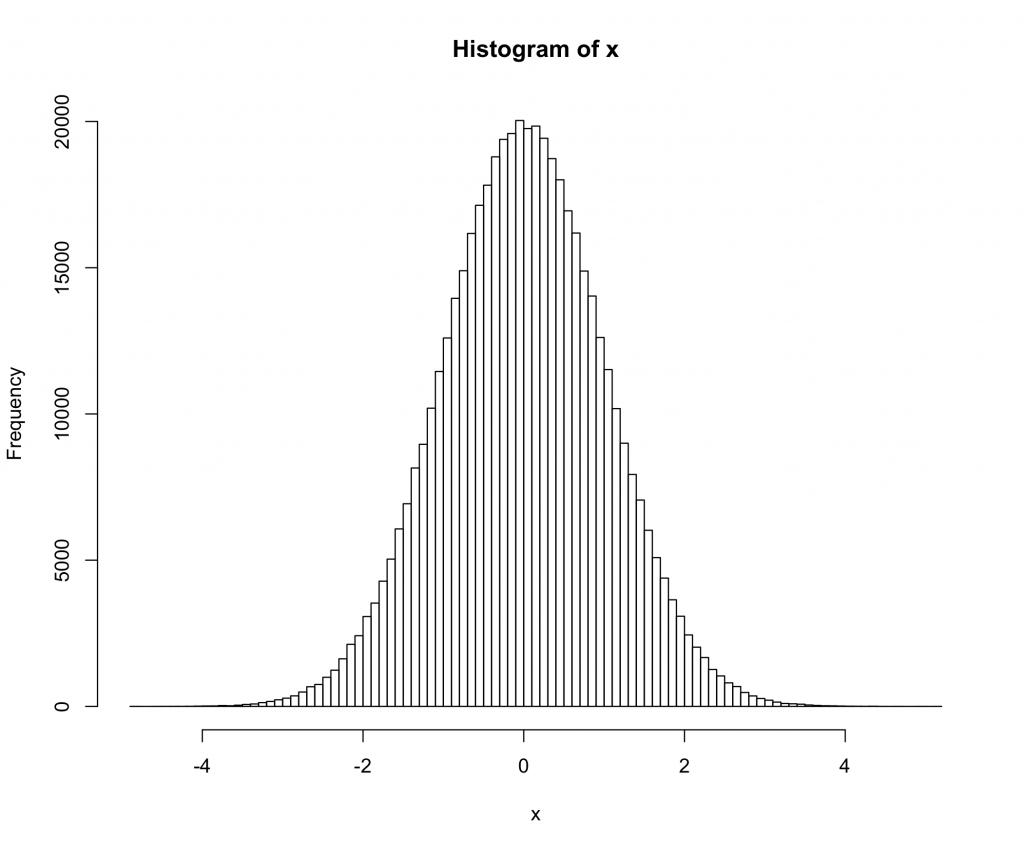
Here we are using a t-distribution with 200 degrees of freedom. The qq-plot shows the distribution is closer to normal than any distribution you are likely to see in the real world, but the test rejects normality with a very high degree of confidence.

Does the significant test against normality mean that we should not use normal theory statistics in this case? (another hint: the answer is no :) )

I would also highly recommend the SnowsPenultimateNormalityTest in the TeachingDemos package. The documentation of the function is far more useful to you than the test itself, though. Read it thoroughly before using the test.

SnowsPenultimateNormalityTest certainly has its virtues, but you may also want to look at qqnorm.

X <- rlnorm(100)
qqnorm(X)
qqnorm(rnorm(100))

Consider using the function shapiro.test, which performs the http://en.wikipedia.org/wiki/Shapiro–Wilk_test">Shapiro-Wilks test for normality. I've been happy with it.

library(DnE)
x<-rnorm(1000,0,1)
is.norm(x,10,0.05)

The Anderson-Darling test is also be useful.

library(nortest)
ad.test(data)

In addition to qqplots and the Shapiro-Wilk test, the following methods may be useful.

Qualitative:

• histogram compared to the normal
• cdf compared to the normal
• ggdensity plot
• ggqqplot

Quantitative:

• nortest package normality tests
• normtest package normality tests

The qualitive methods can be produced using the following in R:

library("ggpubr")
library("car")

h <- hist(data, breaks = 10, density = 10, col = "darkgray") 
xfit <- seq(min(data), max(data), length = 40) 
yfit <- dnorm(xfit, mean = mean(data), sd = sd(data)) 
yfit <- yfit * diff(h$mids[1:2]) * length(data) 
lines(xfit, yfit, col = "black", lwd = 2)

plot(ecdf(data), main="CDF")
lines(ecdf(rnorm(10000)),col="red")

ggdensity(data)

ggqqplot(data)

A word of caution - don't blindly apply tests. Having a solid understanding of stats will help you understand when to use which tests and the importance of assumptions in hypothesis testing.

when you perform a test, you ever have the probabilty to reject the null hypothesis when it is true.

See the nextt R code:

p=function(n){
  x=rnorm(n,0,1)
  s=shapiro.test(x)
  s$p.value
}

rep1=replicate(1000,p(5))
rep2=replicate(1000,p(100))
plot(density(rep1))
lines(density(rep2),col="blue")
abline(v=0.05,lty=3)

The graph shows that whether you have a sample size small or big a 5% of the times you have a chance to reject the null hypothesis when it s true (a Type-I error)